
Part 5 - 입력과 출력 pipeline 디자인하기
Opencv DNN, Tensorflow, Pytorch로 YOLO v3를 구현해본 코드를 보려면 Github repo 를 참고하세요.
본문
지난 Part 4에서는 object confidence 점수와 non-maximum suppression으로 thresholding을 해서 object detect하는 것을 알아봤고, Part 5에서는 실제 detect된 결과를 보여주는 작업을 진행할 예정이다.
해당 코드는 Python 3.5, Pytorch 0.4 에서 실행되게끔 디자인이 되었고, 이 Github repo에서 코드들을 볼 수 있다.
튜토리얼은 총 5 단계로 나뉘어져 있다:
1. Part 1: YOLO가 어떻게 작동되는지 이해하기
2. Part 2 : 네트워크 구조의 layers들 구현하기
3. Part 3 : 네트워크의 forward pass 구현하기
4. Part 4 : Objectness 점수 thresholding과 non-maximum suppression(NMS)
5. Part 5 : 입력과 출력 pipeline 디자인하기
사전에 알아야할 지식
- Part 1~4의 내용
- Pytorch 에 대한 기본 지식,
nn.Module,nn.Sequential,torch.nnparameter class들로 커스텀 구조를 어떻게 구현하는지에 대한 지식도 포함한다. - Opencv 사용법
이번 part에서는 detector의 입력과 출력 pipelines를 구현할 것이다. 이미지를 디스크에서 읽고나서, 예측을 하고, 예측된 결과로 이미지에 bounding box를 그린 다음에 다시 디스크에 저장을 하는 과정이다. 또한, detector로 카메라나 비디오를 실시간으로 처리하는 방법을 다룰 것이다.
Note: Opencv 3이 미리 설치되어있어야 한다.
detect.py 라는 파일을 생성한 후에 필요한 패키지들을 import 한다.
from __future__ import division
import time
import torch
import torch.nn as nn
from torch.autograd import Variable
import numpy as np
import cv2
from util import *
import argparse
import os
import os.path as osp
from darknet import Darknet
import pickle as pkl
import pandas as pd
import random
Creating Command Line Arguments
detect.py 가 detector 실행하는데 사용되는 파일이기 때문에 command line arguments(터미널이나 cmd에서 파일에 전달할 인자들)를 전달하는 것이 좋다. Python의 ArgParse 모듈을 사용해서 해당 기능을 구현했다.
맨위에 --images... 부분을 예시로 각 속성들을 설명해보면:
--images는 이 argument에 해당하는 값을 넣기 원할 때 먼저 나와야 하는 flag이다. Ex)python detect.py --images dog.jpgdest는 argument에 접근할 수 있는 이름이다.args.images로 해당 argument의 값에 접근할 수 있다.help는 단순히 해당 argument가 무엇을 의미하는지 알려주는 역할을 한다.default는 아무 argument를 주지 않았을 때 default의 값을 전달한다는 것을 의미한다.type은 전달 받을 argument의 자료형이다.
def arg_parse():
    """
    Parse arguements to the detect module

    """

    parser = argparse.ArgumentParser(description='YOLO v3 Detection Module')

    parser.add_argument("--images", dest = 'images', help =
                        "Image / Directory containing images to perform detection upon",
                        default = "imgs", type = str)
    parser.add_argument("--det", dest = 'det', help =
                        "Image / Directory to store detections to",
                        default = "det", type = str)
    parser.add_argument("--bs", dest = "bs", help = "Batch size", default = 1)
    parser.add_argument("--confidence", dest = "confidence", help = "Object Confidence to filter predictions", default = 0.5)
    parser.add_argument("--nms_thresh", dest = "nms_thresh", help = "NMS Threshhold", default = 0.4)
    parser.add_argument("--cfg", dest = 'cfgfile', help =
                        "Config file",
                        default = "cfg/yolov3.cfg", type = str)
    parser.add_argument("--weights", dest = 'weightsfile', help =
                        "weightsfile",
                        default = "yolov3.weights", type = str)
    parser.add_argument("--reso", dest = 'reso', help =
                        "Input resolution of the network. Increase to increase accuracy. Decrease to increase speed",
                        default = "416", type = str)

    return parser.parse_args()

args = arg_parse()
images = args.images
batch_size = int(args.bs)
confidence = float(args.confidence)
nms_thesh = float(args.nms_thresh)
start = 0
CUDA = torch.cuda.is_available()
YOLO에서 중요한 argument들로는 images (이미지의 경로), det (detection 결과 저장할 경로), reso (입력 이미지의 resolution, 속도와 nput image's resolution), cfg (configuration 파일 경로) and weightfile(weight 파일 경로) 들이 있다.
Loading the Network
coco.names 파일을 여기서 다운받을 수 있다. 이 파일에는 COCO dataset의 object들의 이름이 들어있다. data 폴더를 작업하고 있는 디렉토리에 만들고 그 안에 저장한다. 해당 작업을 터미널에서 똑같이 진행하려면 밑의 명령어만 작성해도 된다.
mkdir data
cd data
wget https://raw.githubusercontent.com/ayooshkathuria/YOLO_v3_tutorial_from_scratch/master/data/coco.names
그 다음에 class 파일을 load한다.
num_classes = 80    #For COCO
classes = load_classes("data/coco.names")
load_classes 는 util.py 에 정의된 함수인데, 각 class의 index와 이름을 dictionary 형태로 만든 다음에 리턴한다.
def load_classes(namesfile):
    fp = open(namesfile, "r")
    names = fp.read().split("\n")[:-1]
    return names
네트워크를 초기화하고 weights를 load한다.
#Set up the neural network
print("Loading network.....")
model = Darknet(args.cfgfile)
model.load_weights(args.weightsfile)
print("Network successfully loaded")

model.net_info["height"] = args.reso
inp_dim = int(model.net_info["height"])
assert inp_dim % 32 == 0
assert inp_dim > 32

#If there's a GPU availible, put the model on GPU
if CUDA:
    model.cuda()

#Set the model in evaluation mode
model.eval()
Read the Input images
이미지를 디스크 혹은 디렉토리에서 읽어들인다. 이미지의 경로들은 리스트 형식의 imlist 저장되어 있다.
read_dir = time.time()
#Detection phase
try:
    imlist = [osp.join(osp.realpath('.'), images, img) for img in os.listdir(images)]
except NotADirectoryError:
    imlist = []
    imlist.append(osp.join(osp.realpath('.'), images))
except FileNotFoundError:
    print ("No file or directory with the name {}".format(images))
    exit()
read_dir 은 시간을 측정하는데 사용되는 checkpoint이다. (앞으로도 여러번 나온다)
만약 det flag에 정의된 detection된 결과를 저장할 디렉토리가 없다면 해당 폴더를 생성한다.
if not os.path.exists(args.det):
    os.makedirs(args.det)
OpenCV를 사용해서 이미지를 load한다.
load_batch = time.time()
loaded_ims = [cv2.imread(x) for x in imlist]
load_batch 는 checkpoint이다.
OpenCV 는 이미지를 numpy array 형태로 load하고 채널의 순서는 BGR(우리가 흔히 말하는 RGB와 순서가 반대다)이다. Pytorch의 입력 이미지 형태는 (Batches x Channels x Height x Width)이고 채널의 순서는 RGB이다. 이러한 차이 때문에 numpy array를 Pytorch 입력 이미지 형태로 변형해야한다. utils.py 파일에 해당 역할을 수행하는 prep_imag함수를 작성할 것이다.
다만 prep_image 함수를 작성하기 전에 letterbox_image 라는 함수를 정의해야 한다. 이 함수는 이미지 비율을 유지하고 남은 영역을 (128,128,128)로 채운 상태로 이미지를 resize한다.
def letterbox_image(img, inp_dim):
    '''resize image with unchanged aspect ratio using padding'''
    img_w, img_h = img.shape[1], img.shape[0]
    w, h = inp_dim
    new_w = int(img_w * min(w/img_w, h/img_h))
    new_h = int(img_h * min(w/img_w, h/img_h))
    resized_image = cv2.resize(img, (new_w,new_h), interpolation = cv2.INTER_CUBIC)

    canvas = np.full((inp_dim[1], inp_dim[0], 3), 128)

    canvas[(h-new_h)//2:(h-new_h)//2 + new_h,(w-new_w)//2:(w-new_w)//2 + new_w,  :] = resized_image

    return canvas
이제 OpenCV 이미지를 받아들여서 네트워크의 입력으로 사용될 수 있게 형태를 변형하는 prep_image 함수를 작성한다.
def prep_image(img, inp_dim):
    """
    Prepare image for inputting to the neural network.

    Returns a Variable
    """

    img = cv2.resize(img, (inp_dim, inp_dim))
    img = img[:,:,::-1].transpose((2,0,1)).copy()
    img = torch.from_numpy(img).float().div(255.0).unsqueeze(0)
    return img
이미지를 변형한 후에 원본 이미지를 im_dist_list에 저장한다.
#PyTorch Variables for images
im_batches = list(map(prep_image, loaded_ims, [inp_dim for x in range(len(imlist))]))

#List containing dimensions of original images
im_dim_list = [(x.shape[1], x.shape[0]) for x in loaded_ims]
im_dim_list = torch.FloatTensor(im_dim_list).repeat(1,2)

if CUDA:
    im_dim_list = im_dim_list.cuda()
Create the Batches
leftover = 0
if (len(im_dim_list) % batch_size):
   leftover = 1

if batch_size != 1:
   num_batches = len(imlist) // batch_size + leftover
   im_batches = [torch.cat((im_batches[i*batch_size : min((i +  1)*batch_size,
                       len(im_batches))]))  for i in range(num_batches)]
The Detection Loop
Batch를 iterate하면서 prediction을 하고 detection을 해야하는 모든 이미지의 prediction tensor들(write_output 함수의 output으로 D x 8의 모양이다)을 concatenate 한다.
Batch 마다, 입력을 받고 나서 write_results 함수를 통해 output 값이 얻어지는데 걸리는 시간을 detection 시간으로 간주한다. write_results 에 의해 리턴된 output의 attribute(특성) 중에는 batch내 이미지의 index가 있었다. 이 index를 transform(변형)해서 imlist (전체 이미지의 주소를 가지고 있는 리스트)내 이미지의 index를 나타내게 한다.
그 다음에는 detection하는데 걸린 시간과 이미지마다 detect된 object를 print 한다.
write_results 함수의 리턴 값이 int (0) 이면 detection이 없다는 의미이기 때문에, continue 를 사용해서 loop의 나머지 부분을 건너뛴다.
write = 0
start_det_loop = time.time()
for i, batch in enumerate(im_batches):
    #load the image
    start = time.time()
    if CUDA:
        batch = batch.cuda()

    prediction = model(Variable(batch, volatile = True), CUDA)

    prediction = write_results(prediction, confidence, num_classes, nms_conf = nms_thesh)

    end = time.time()

    if type(prediction) == int:

        for im_num, image in enumerate(imlist[i*batch_size: min((i +  1)*batch_size, len(imlist))]):
            im_id = i*batch_size + im_num
            print("{0:20s} predicted in {1:6.3f} seconds".format(image.split("/")[-1], (end - start)/batch_size))
            print("{0:20s} {1:s}".format("Objects Detected:", ""))
            print("----------------------------------------------------------")
        continue

    prediction[:,0] += i*batch_size    #transform the atribute from index in batch to index in imlist

    if not write:                      #If we have't initialised output
        output = prediction
        write = 1
    else:
        output = torch.cat((output,prediction))

    for im_num, image in enumerate(imlist[i*batch_size: min((i +  1)*batch_size, len(imlist))]):
        im_id = i*batch_size + im_num
        objs = [classes[int(x[-1])] for x in output if int(x[0]) == im_id]
        print("{0:20s} predicted in {1:6.3f} seconds".format(image.split("/")[-1], (end - start)/batch_size))
        print("{0:20s} {1:s}".format("Objects Detected:", " ".join(objs)))
        print("----------------------------------------------------------")

    if CUDA:
        torch.cuda.synchronize()
torch.cuda.synchronize CUDA kernel이 CPU와 synchronize(동기화)되게 한다. 만약 동기화를 하지 않는다면, CUDA kernel은 GPU 작업이 queue되자마자 그리고 GPU 작업이 끝나기도 전에 CPU에게 control을 주게 된다(비동기적 호출). 그렇게 되면 end=time.time() 이 GPU 작업이 끝나지도 않았는데도 print되서 왜곡된 시간 결과가 나올 수 있게 된다.
이제 Tensor Output에 모든 이미지에 대한 detection을 갖게 되고 이제 bouding box들을 이미지에 그리면 된다.
Drawing bounding boxes on images
Try-catch 블록을 사용해서 detection이 하나라도 있는지 확인을 한다. 만약 detection이 하나도 안되었다면 프로그램을 종료한다.
try:
    output
except NameError:
    print ("No detections were made")
    exit()
Prediction인 output tensor는 네트워크의 입력 크기에 대응되지만 원본 이미지 크기에는 대응되지 않는다. 그래서, bounding box들을 그리기 전에 다시 output을 transform(변환)해야 한다. Bounding box의 꼭지점 좌표들을 원본 이미지에 맞게 변환을 한다.
im_dim_list = torch.index_select(im_dim_list, 0, output[:,0].long())

scaling_factor = torch.min(416/im_dim_list,1)[0].view(-1,1)


output[:,[1,3]] -= (inp_dim - scaling_factor*im_dim_list[:,0].view(-1,1))/2
output[:,[2,4]] -= (inp_dim - scaling_factor*im_dim_list[:,1].view(-1,1))/2
위 코드를 통해서 원본 이미지에 맞도록 좌표들을 변환했다. 하지만, letterbox_image함수에서 이미지의 dimension을 scaling factor에 의해 resize를 했었다 (비율을 유지하기 위해 공통된 factor로 나뉘었었다). 그래서 rescaling 취소해서 bouding box의 원본 이미지에서의 좌표를 구한다.
output[:,1:5] /= scaling_factor다음으로는, 이미지 바깥에 boundary를 가지는 bounding box를 잘라서 이미지 내에 edge들이 있게 한다.
for i in range(output.shape[0]):
    output[i, [1,3]] = torch.clamp(output[i, [1,3]], 0.0, im_dim_list[i,0])
    output[i, [2,4]] = torch.clamp(output[i, [2,4]], 0.0, im_dim_list[i,1])
Bounding box들이 한 이미지 내에 너무 많으면 모든 box들을 한가지 색상으로 칠하는 것은 좋은 생각이 아닐 수 있다. 이 파일을 다운받아서 작업하는 디렉토리에 넣는다. 이 파일을 pickled(객체를 있는 그대로 저장한 포맷) 파일이고 여러 색상들에 대한 정보를 가지고 있고 이 정보들을 사용해서 랜덤하게 box를 색칠할 예정이다.
output_recast = time.time()
class_load = time.time()
colors = pkl.load(open("pallete", "rb"))
Box를 그리는 함수이다.
draw = time.time()


def write(x, results):
    c1 = tuple(x[1:3].int())
    c2 = tuple(x[3:5].int())
    img = results[int(x[0])]
    cls = int(x[-1])
    color = random.choice(colors)
    label = "{0}".format(classes[cls])
    cv2.rectangle(img, c1, c2,color, 1)
    t_size = cv2.getTextSize(label, cv2.FONT_HERSHEY_PLAIN, 1 , 1)[0]
    c2 = c1[0] + t_size[0] + 3, c1[1] + t_size[1] + 4
    cv2.rectangle(img, c1, c2,color, -1)
    cv2.putText(img, label, (c1[0], c1[1] + t_size[1] + 4), cv2.FONT_HERSHEY_PLAIN, 1, [225,255,255], 1);
    return img
위 함수는 colors 에서 랜덤하게 색상을 뽑아서 box를 그린다. Box위에는 작은 box 하나를 더 생성해서 detect된 class의 이름을 표시한다. cv2.rectangle의 -1 argument는 box를 색상으로 fill하는 작업을 한다.
이 write 함수를 로컬에 정의를 해서 colors 리스트를 접근할 수 있도록 했다. 함수를 정의했으니 이제 bounding box를 이미지에 그리는 작업을 한다.
list(map(lambda x: write(x, loaded_ims), output))

det_names = pd.Series(imlist).apply(lambda x: "{}/det_{}".format(args.det,x.split("/")[-1]))
위 lambda 코드는 loaded_ims 에 있는 이미지를 write 함수에 보내고 리턴 받은 값을 리스트로 저장한다.
이미지는 det_이미지이름 의 형태로 저장을 한다. Address의 리스트를 생성해서 detect된 이미지를 저장한다.
마지막으로, det_names (저장할 장소에 대한 argument)에다 이미지들을 저장한다.
list(map(cv2.imwrite, det_names, loaded_ims))
end = time.time()
Printing Time Summary
Detector 맨 마지막에는 지금까지 진행한 코드의 실행시간에 대한 내용을 print한다. 각 파트마다의 실행시간을 보면서 어떤 hyperparamter가 detector의 속도에 영향을 끼치는지 알 수 있게 된다. Hyperparameters는 batch 크기, objectness confidence 그리고 NMS threshold(각각 bs, confidence, nmx_threshold 라는 flag로 전달된다)는 프로그램 시작할 때 command line에서 설정을 변경할 수 있다.
print("SUMMARY")
print("----------------------------------------------------------")
print("{:25s}: {}".format("Task", "Time Taken (in seconds)"))
print()
print("{:25s}: {:2.3f}".format("Reading addresses", load_batch - read_dir))
print("{:25s}: {:2.3f}".format("Loading batch", start_det_loop - load_batch))
print("{:25s}: {:2.3f}".format("Detection (" + str(len(imlist)) +  " images)", output_recast - start_det_loop))
print("{:25s}: {:2.3f}".format("Output Processing", class_load - output_recast))
print("{:25s}: {:2.3f}".format("Drawing Boxes", end - draw))
print("{:25s}: {:2.3f}".format("Average time_per_img", (end - load_batch)/len(imlist)))
print("----------------------------------------------------------")


torch.cuda.empty_cache()
Testing The Object Detector
터미널 혹은 cmd에서 해당 프로그램을 실행시키려면 다음과 같은 명령어를 작성한다
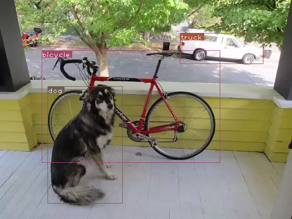
python detect.py --images dog-cycle-car.png --det det현 코드는 CPU에서 실행이 되었다. GPU에서는 detection 시간이 더 빠를 것으로 예상된다. Tesla K80에서는 이미지당 0.1초 정도 걸린다.
Loading network.....
Network successfully loaded
dog-cycle-car.png    predicted in  2.456 seconds
Objects Detected:    bicycle truck dog
----------------------------------------------------------
SUMMARY
----------------------------------------------------------
Task                     : Time Taken (in seconds)

Reading addresses        : 0.002
Loading batch            : 0.120
Detection (1 images)     : 2.457
Output Processing        : 0.002
Drawing Boxes            : 0.076
Average time_per_img     : 2.657
----------------------------------------------------------
det_dog-cycle-car.png 라는 이미지 파일이 det 디렉토리에 저장이 된다.
Running the Detector on Video/Webcam
Detector를 비디오나 웹캠에서 실행시키기 위해서, 대부분의 코드는 비슷하지만, batch를 iterate할 필요가 없어진다.
비디오를 실행시키는 코드는 Github repo의 video.py 에 있다. detect.py 와 거의 유사하나 약간의 변화가 있다.
처음에 비디오 / 웹캠을 OpenCV에서 작동시킨다.
videofile = "video.avi" #or path to the video file.

cap = cv2.VideoCapture(videofile)

#cap = cv2.VideoCapture(0)  for webcam

assert cap.isOpened(), 'Cannot capture source'

frames = 0
이미지를 iterate했던 것 처럼 비디오의 frame들을 iterate한다.
Batch를 다룰 필요가 없어졌고 한 타임에 하나의 이미지만 처리하면 되기 때문에 많은 양의 코드가 단순하게 바뀌었다. 여러 이미지가 한번에 오는 것이 아니라 한 frame을 읽을 때마다 하나의 이미지만 읽을 수 있기 때문에 그렇다. 이러한 이유 때문에 im_dim_list를 사용하는 대신에 tuple을 사용하게 되었고, write 함수에도 약간의 변화가 생겼다.
각 iteration 마다, 몇 개의 frame이 지났는지에 대한 정보를 frames 라는 변수에 담는다. 비디오가 다 읽히고 나서 총 실행시간을 frame으로 나눠서 비디오의 FPS를 구한다.
Detection 이미지를 디스크에 저장하는 cv2.imwrite대신에, cv2.imshow 를 사용해서 bounding box가 그려진 frame을 보여준다. 유저가 Q 버튼을 누르면 loop에서 빠져나오고 비디오를 중단한다.
frames = 0
start = time.time()

while cap.isOpened():
    ret, frame = cap.read()

    if ret:
        img = prep_image(frame, inp_dim)
#        cv2.imshow("a", frame)
        im_dim = frame.shape[1], frame.shape[0]
        im_dim = torch.FloatTensor(im_dim).repeat(1,2)

        if CUDA:
            im_dim = im_dim.cuda()
            img = img.cuda()

        output = model(Variable(img, volatile = True), CUDA)
        output = write_results(output, confidence, num_classes, nms_conf = nms_thesh)


        if type(output) == int:
            frames += 1
            print("FPS of the video is {:5.4f}".format( frames / (time.time() - start)))
            cv2.imshow("frame", frame)
            key = cv2.waitKey(1)
            if key & 0xFF == ord('q'):
                break
            continue
        output[:,1:5] = torch.clamp(output[:,1:5], 0.0, float(inp_dim))

        im_dim = im_dim.repeat(output.size(0), 1)/inp_dim
        output[:,1:5] *= im_dim

        classes = load_classes('data/coco.names')
        colors = pkl.load(open("pallete", "rb"))

        list(map(lambda x: write(x, frame), output))

        cv2.imshow("frame", frame)
        key = cv2.waitKey(1)
        if key & 0xFF == ord('q'):
            break
        frames += 1
        print(time.time() - start)
        print("FPS of the video is {:5.2f}".format( frames / (time.time() - start)))
    else:
        break
Conclusion
5개의 튜토리얼을 통해서 YOLO object detector를 처음부터 구현을 해봤다. 딥러닝을 가장 배우기 좋은 방법은 직접 코드로 구현을 해보는 것이다. 구현을 하다보면 논문에서 지나친 개념들에 대한 정보들을 다시 돌아볼 수 있게 한다. 이 튜토리얼이 딥러닝을 공부하는데 좋은 경험이 되기를 바란다.
Further Reading
소감문
이로써 5파트에 나뉜 YOLO object detector를 구현하는 튜토리얼이 끝났다. 본인은 튜토리얼을 따라하면서 직접 코드를 구현해봤고, 이 저자의 코드 뿐만 아니라 다른 사람들의 코드도 사용해봤다. 같은 논문에 대한 내용을 코드로 구현했지만 방식이 제법 달랐다. 그리고 실행속도 측면에서도 코드를 어떻게 짜느냐에 따라서 많이 달랐다.
실행결과 이 post 저자의 코드보다 다른 저자의 코드가 속도면에서 더 빨랐다. 그 코드를 분석해보면 이 post 저자의 코드보다 조금 더 간결하게 작성됬음을 알 수 있다. 더 빠른 YOLO 코드를 참고하고 github repo 여기를 참고하면 된다.